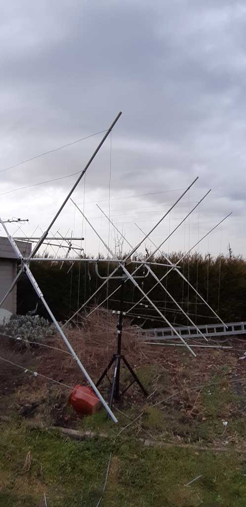
Modelling, building and measuring a 4 element Dual Band Cubical Quad antenna (6m-4m).
Methodology adopted :
1st Step :
Model with MMANA-GAL software the existing descriptions of the 4 elements cubical quad antennas given into the publications of L.B. Cebik (W4RNL), William I.Orr (W6SAI), Carl O. Jelinek N6VNG.
The modelling-based antennas gived very similar results. Each model have been optmized several times.
The here given dimensions below are derived from the several opizations (gain, F/B/ SWR) made with MMANA-GAL software.
Perimeter of the loops (in mm)
| REFLECT. | RAD. | D1 | D2 | |
| 50.2MHz | 6288 | 6128 | 5740 | 5753 |
| 70.2 MHz | 4616 | 4436 | 4356 | 4292 |
Spacing REFL.-D2 = 2752 mm
=> : Download the MMANA-GAL file here (right mouse button: save as)
(*) MMANA-GAL users : for 50.2 MHz source w11c - for 70.2 MHz source w17c
Settings MMANA-GAL :
- Calculation above real ground (not on freespace); soil conductivity chosen with world atlas of conductivities (World atlas of ground conductivities (hamwaves.com)). I make a modelling above real ground because I do my measurements above a real ground. (Now,... if the NASA wants to take to the space my antennas for free and make my measurements, I have no objection!)
- I set a soil conductivity of 30 mS/m (just of curiosity, I made modelling with other conductivity values,there was little difference between the results, excepted for sea water)
- Antenna height : 7 mètres
- Wire jauge for the loops : fence aluminium wire diameter 2 mm
- Modelling doesn't include the boom, cross arms structure,loop roots, mast and roof. Many modelling have been made with/without those neighbouring objects with little difference into the results, so I didn't included them.
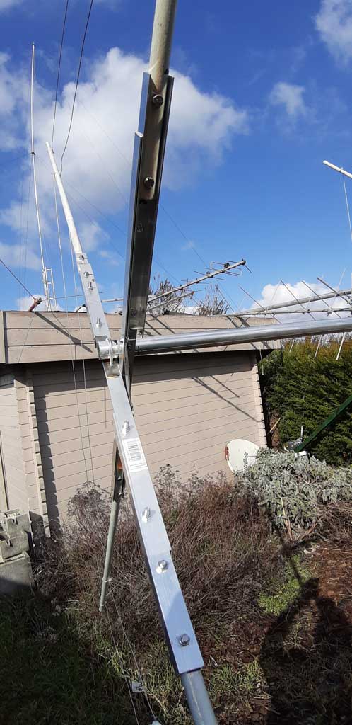
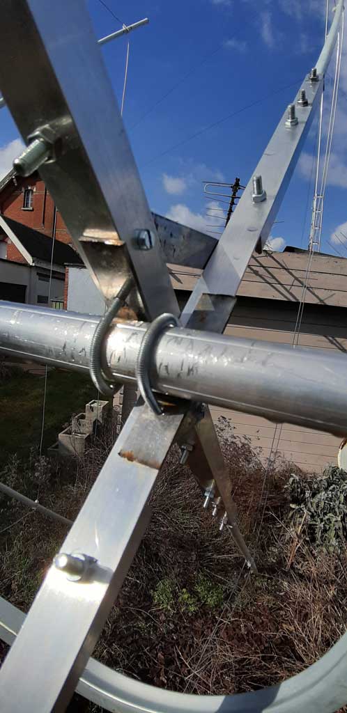
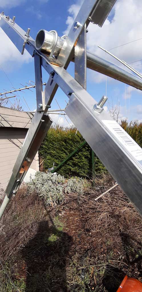
Step 2 : building the antenna
The hardware is coming from a hobby store.
Cross arms and structure are made with aluminium corners and "U" profiles,In order to ensure that the cross arms are square and reinforced, I use flat iron strip 1 cm wide, they will be painted and coated with epoxy resin.
Screews and bolts are M5 satinless steel.
Aluminium fence wire 2 mm diameter
Roots are made with hardwood dowel dia.12mm, painted and coated with epoxy resin.
Step 3 : MMANA-GAL modelling, NanoVNA measurements & compare the results
Loop 50.2 MHz
Modelling MMANA-GAL
NanoVNA measuring conditions fully respecting the conditions set for the modelling
• Device Under Test (DUT) height : 7 m
• Neighbouring objects at least 10m from the DUT
• VNA connected directly to the loop , connection the computer via a 10 meter USB cable.
• Software nano-VNA Saver v 0.2.2
• VNA calibration :
• STIMULUS START : 49.5 MHz
• STIMULUS STOP :51.0 MHz
• CALIBRATION : RESET – CH0 OPEN – CH0 SHORT – CH0 LOAD – CH0 ISOLN (NO LOAD) + CH1 I(LOAD)
• SAVE 0
• Connectors SMA + adapter -> N (is included into the calibration)
MEASUREMENTS @50.2 MHz
• Sweep start : 49.5 MHz
• Sweep stop : 51 MHz
Impedance : Software v/s Measurement @50.2 MHz• MMANAGAL : 50.2-j0.0253 Ω • Mesure NanoVNA : 50.69+j.0759 Ω |
Plots MMANA-GAL and impedances from 49.95MHz to 50.45MHz
Software results v/s measured values
| Freq (MHz) | MMANA—GAL | NanoVNA |
| 49.95 | 45.3 - j12.2 Ω | 45.57 - j10 Ω |
| 50.075 | 47.8 - j6 Ω | 48.11 - j4.79 Ω |
| 50.2 | 50.2 - j0.0253 Ω | 50.69 + j0.759 Ω |
| 50.325 | 52.6 + j5.5 Ω | 53.41 + j6.41 Ω |
| 50.45 | 54.9 + j10.9 Ω | 56.51 + j12.3 Ω |
MMANA-GAL : resonance
NanoVNA : resonance measurement
Resonance : software v/s measurement @50.2 MHz
|
MMANA-GAL |
F.RES 50.203 MHZ | Z = 50.2 - j253 10-4 Ω |
| NANOVNA | F.RES 50.186 MHZ | Z = 50.41 – j876 10-4 Ω |
Smith Chart (SWR circles included)
MMANAGAL : SWR curve
NanoVNA : SWR measurement
Software: Forward Gain (DBi) & F/B (dB)
LOOP 70.2 MHz
Modelling MMANA-GAL
NanoVNA measuring conditions fully respecting the conditions set for the modelling
• Device Under Test (DUT) height : 7 m
• Neighbouring objects at least 10m from the DUT
• VNA connected directly to the loop , connection the computer via a 10 meter USB cable.
• Software nano-VNA Saver v 0.2.2
• VNA calibration :
• STIMULUS START : 69 MHz
• STIMULUS STOP :72.0 MHz
• CALIBRATION : RESET – CH0 OPEN – CH0 SHORT – CH0 LOAD – CH0 ISOLN (NO LOAD) + CH1 I(LOAD)
• SAVE 0
• Connectors SMA + adapter -> N (is included into the calibration)
MEASUREMENTS @70.2 MHz
• Sweep start : 69.0 MHz
• Sweep stop : 72.0 MHz
Impedance : sotfware v/s measurement @70.2MHz· MMANA-GAL : 50.2-j0.0253 Ω
· Mesure NanoVNA : 12.57+j.2.84 Ω
|
Plots MMANA-GAL and impedances from 69 MHZ to 72 MHz
Software results v/s measured values
| Freq (MHz) | MMANAG—GAL |
|
|
| 69.8 | 63.3 – j13.0 Ω | 11.48 - j16 Ω | |
| 70.0 | 56.8 – j8.5 Ω | 12.22 – j7.15 Ω | |
| 70.2 | 48.7 – j2.2 Ω | 12.57 + j2.4 Ω | |
| 70.4 | 39.6 + j6.8 Ω | 13.31 + j13.8 Ω | |
| 70.6 | 30.6 + j18.6 Ω | 14.31 + j25.8 Ω |
MMANA-GAL : resonance
NanoVNA : resonance measurement
Marker @70.167 MHz
Résonance : software v/s measurement
| MMANA-GAL | F.RES 70.274 MHZ | Z = 45.37 – j0.8206 Ω | |
| NanoVNA | F.RES 70.1476 MHZ | Z = 12.45 – j34 10-4 Ω |
Abaque de Smith :
Marker @70.167 MHz
Software : SWR
NanoVNA : SWR measurement
Software : Forward Gain (DBi) & F/B (dB)
REMARKS :
- @70.2 MHz a clear differnce about impedance (&SWR) is observed between software results and measurements
- About resonance there is a ∆=126KHZ between software results and measurements,
- I observed in several calculations @70.2 MHz, if I leaved the 50 MHZ loop open, there was a difference in regard of the same modelling with the 50 MHz loop closed.
- Inversely, in calculations @50.2 MHz this difference is not so important(see table below)
calculation 3 @50.2 MHz with 70 MHz loop open
calculation 4 @50.2 MHz with 70 MHz loop closed
I have no explanation (not yet) but
she would like to know a re-modelling of this antenna with other softwares (NEC, 4NEC2) and see if whe have the same differnces.
In the present study case, this antenna is principaly purposed to be used on the begining of the 6 meter band, the use of the 4 meter band constitutes a balanced and realistic compromise about forward gain and F/B ratio (this applies for all the multiband cubal quad using common loops).
STEP 4 : feeding the antenna
FEEDING THE 50.2 MHz LOOP
The measured SWR for the 6m band is 1.02:1 thus a balancing of the antenna feed system is only needed to avoid a disorsion of the Far field pattern due to the unbalance of the coaxial cable.
Easy UNBAL to BAL solutions
- Use 1 :1 UN/BAL current balun
- Use a gamma match
- Use coaxial stubs
I used coaxial stubs.
Illustration : (from ARRL Antenna Book)
How it works :
The purpose is to obtain 2 currents in opposed phase to feed the loop. We send simultany a current trough 2 coaxial lines, the second coax line is 1/2 wave (180°) longer, so the current is 1/2wave (180°) later then the current into the first coax line. The 2 currents are phased 180° each of other.
After installation of those stubs on the antenna, I re-measured all on 50.2 MHz : resonance & SWR remains unchanged.
A alterned method.
FEEDING THE 70.2 MHz LOOP
The gamma match method adapt the impedance and balance the feed of the loop.
To calculate tour gamma match see link :
Microsoft Word - N6MWGamma4.doc (nonstopsystems.com)
Figure and dimensions
Note :
Diameter of both wires are identical.(aluminium fence wire diameter 2mm).
The variable condensator can be replaced by a open piece of coaxial cable .
The value of C (pF/m) is given by the cable manufacturer or can be measured with a capacimeter.
STEP 5 : Measurement of the antenna patern & antenna Gain
Measuring the antenna patern
I use for this a software called Polarplot created by G4HFQ , it can be dowloaded here G4HFQ Radio Programming Software .
Al the explanations are given in the help file of the program.
How I used Polarplot.
I have taken h = 1λ & D = 10λ
There are other many methods.
Example: Relevé du diagramme de rayonnement d'une antenne yagi 144 (pagesperso-orange.fr)
You can use your DIY field meter, thsi will give you already a good evaluation of your antenna caracteristics.
Best 73's ON8IM